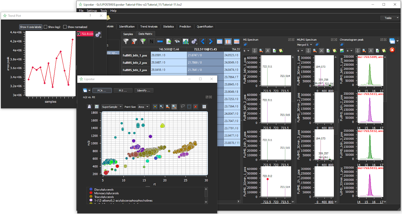
Lipostar2 is a comprehensive, vendor-neutral software for LC-MS/MS-based lipidomics (DDA and DIA), which includes a large number of features including: raw data import and peak detection, identification, quantification, statistical analysis, trend analysis and biopathways analysis.
Lipostar2 finds application in untargeted and semi-targeted lipidomics, including stable isotope labelling experiments. Within a Lipostar session, different modes of lipidomics analysis can be combined to increase knowledge and obtain a more comprehensive analysis of lipid profiles.
Key features
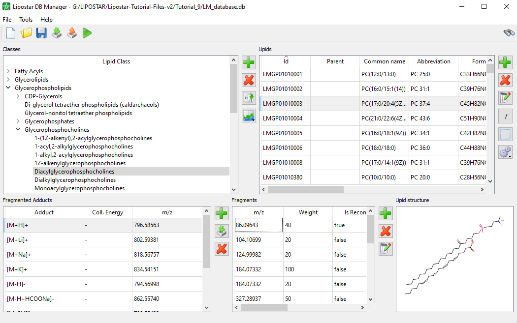
- The DB Manager module that enables the generation of databases of fragmented lipids by applying fragmentation rules provided by the software or by importing experimental MS/MS data
- A flexible lipid identification approach that includes:
- a spectral matching approach
- high-throughput bottom-up approach, based on class-specific fragment recognition
- high-throughput identification of oxidized species.
- A gap-filler algorithm to reduce missing values
- Various plots to visualize and refine identification results
- Various multivariate statistical analysis tools
- Lipid pathways
Suggested computer configuration
- PC with Windows 10, 11 64bit
- Minimum 16Gb of RAM required
- Suggested 32/64Gb of RAM and large SSD to store raw files, compound DBs, and sessions
Data Processing
- More instruments supported. Now Lipostar 2 reads the most common file formats:
- Agilent Q-Tof(*.d): AutoMS and full scan at multiple energies of collision (All Ions).
- Waters (*.raw): MSe, HDMSe, DDA, and MSMS, SONAR
- Thermo-Fisher (*.RAW): Ion-Trap and Orbitrap, Exactive, Q-Exactive, DDA and AIF
- ABSCiex *.wiff file format.
- Bruker (*.d): QTof, FT-ICR, TIMS-TOF data dependent scan.
- Shimadzu (*.lcd): QTof
- Data processing can be run in the background.
Data Analysis
- Trend analysis for global lipid profiling
Identification
- New fragmentation rules for automatic lipid identification
- Lipid database generation from in-house data
- Improved adduct and in source fragmentation clustering
- Customized adducts support
- Transfer of identification results to submatrices
- Kendrick mass defect plot
- Use of Waters CCS values for identification scores
Quantification
- New handling of adduct information
Lipid pathways
- Updated and new biopathways maps available (metabolism & disease)
Cross-talk with other software
- Connection to LipidLynxX for lipid annotation
- connection to LPPTiger for in depth identification of oxidized species
Lipostar Training documents. Version 2.2.1
- Tutorial_Lipostar2 Appendix
- Tutorial_Lipostar2 Manual
- Tutorial_Lipostar2_01 Select your style before start
- Tutorial_Lipostar2_02 The Lipostar DB manager
- Tutorial_Lipostar2_03 Generating a database of in-house data
- Tutorial_Lipostar2_04 The Lipid Builder in DB Manager
- Tutorial_Lipostar2_05 First steps into Lipostar
- Tutorial_Lipostar2_06 Search for drug metabolites in data matrix
- Tutorial_Lipostar2_07 Lipostar for Flux analysis
- Tutorial_Lipostar2_08 Exploring lipid pathways
- Tutorial_Lipostar2_09 Lipid quantification
- Tutorial_Lipostar2_10 Normalization in Lipostar
- Tutorial_Lipostar2_11 The trend analysis: filtering global profiling lipidomics data by anticipated trends
- Tutorial_Lipostar2_12 Grouping adducts and in source fragments
- Tutorial_Lipostar2_13 Data export and report generation
- Tutorial_Lipostar2_14 Additional features and tools
- Tutorial_Lipostar2_15 Ion Mobility Spectrometry (IMS) data analysis
- Tutorial_Lipostar2_16 Waters DDA data
Articles:
- Lipidomics‐Guided Ultrasound‐Assisted Ethanol Extraction of Avocado Pulp and Evaluation of Bioactive Properties
- September 30, 2025. Bruna B. Neves, Rita Pais, Joana Batista, Marisa Pinho, Tatiana Maurício, Stefano Bonciarelli, Laura Goracci, Bruno Neves, Pedro Domingues, M. Rosário Domingues, Tânia Melo
- Rediscovering Halophyte Suaeda maritima as an Alternative crop for Food Lipids Through Aquaponic Cultivation and Lipidomics analysis
- September 24, 2025. Marisa Pinho, Ana S. P. Moreira, Erika García Cardesín, Alexandra Pérez-González, David Gómez-Carnota, Bruna B. Neves, Stefano Bonciarelli, Laura Goracci, Tânia Melo, Pedro Domingues, Ana I. Lillebø, Javier Cremades, M. Rosário Domingues
- Lipidomic Profiling of Red Blood Cells in the Mitochondrial Fatty Acid β-oxidation Disorder MCADD Reveals Phospholipid and Sphingolipid Dysregulation
- July 24, 2025. Inês M. S. Guerra, Helena B. Ferreira, Luísa Diogo, Sónia Moreira, Stefano Bonciarelli, Laura Goracci, Tânia Melo, Pedro Domingues, M. Rosário Domingues, Ana S. P. Moreira
- Unveiling the lipidomic profile of aerial plant and seed of the halophyte Suaeda albescens and their bioactive properties for food and nutraceutical applications
- June 17, 2025. Marisa Pinho, Francisca Marques, Inês M. S. Guerra, Ana Moreira, Tânia Melo, Stefano Bonciarelli, Laura Goracci, Pedro Domingues, Ana I. Lillebø, Javier Cremades, M. Rosário Domingues
- LC-MS and High-Throughput Data Processing Solutions for Lipid Metabolic Tracing Using Bioorthogonal Click Chemistry
- 24 April 2025. Palina Nepachalovich, Stefano Bonciarelli, Gabriele Lombardi Bendoula, Jenny Desantis, Michela Eleuteri, Christoph Thiele, Laura Goracci, Maria Fedorova
- Phosphatidylethanolamine species with n-3 and n-6 fatty acids modulate macrophage lipidome and attenuate responses to LPS stimulation
- April 2025. Tatiana Maurício, Inês M. S. Guerra, Marisa Pinho, Tânia Melo, Stefano Bonciarelli, Laura Goracci, Bruno Neves, Rosário Domingues, Pedro Domingues
- Unmasking the lipid landscape: carbamazepine induces alterations in Leydig cell lipidome
- February 2025. Inês Nobre, Inês M. S. Guerra, Marisa Pinho, Ana D. Martins, Laura Goracci, Stefano Bonciarelli, Tânia Melo, Pedro Domingues, Artur Paiva, Pedro F. Oliveira, M. Rosário Domingues
- Plasma lipidomics analysis reveals altered profile of triglycerides and phospholipids in children with Medium-Chain Acyl-CoA dehydrogenase deficiency
- July 2024. Inês M S Guerra, Helena B Ferreira, Tatiana Maurício, Marisa Pinho, Luísa Diogo, Sónia Moreira, Laura Goracci, Stefano Bonciarelli, Tânia Melo, Pedro Domingues, M Rosário Domingues, Ana S P Moreira
- A platelet lipidomics signature in patients with COVID-19
- December 2023. Laura Goracci, Eleonora Petito, Alessandra Di Veroli, Emanuela Falcinelli, Caterina Bencivenga, Elisa Giglio, Cecilia Becattini, Edoardo De Robertis, Gaetano Vaudo, Paolo Gresele
- Analysis of Phosphatidylinositol Modifications by Reactive Nitrogen Species Using LC-MS: Coming to Grips with Their Nitroxidative Susceptibility
- July 2023. Stefano Bonciarelli, Bruna Neves, Pedro Domingues, Tânia Melo, Laura Goracci, Maria Rosário Domingues
- Guiding the choice of informatics software and tools for lipidomics research applications
- February 2023. Zhixu Ni , Michele Wölk, Geoff Jukes, Karla Mendivelso Espinosa, Robert Ahrends, Lucila Aimo, Jorge Alvarez-Jarreta, Simon Andrews, Robert Andrews, Alan Bridge, Geremy C Clair, Matthew J Conroy, Eoin Fahy, Caroline Gaud, Laura Goracci, Jürgen Hartler, Nils Hoffmann, Dominik Kopczyinki, Ansgar Korf, Andrea F Lopez-Clavijo, Adnan Malik, Jacobo Miranda Ackerman, Martijn R Molenaar, Claire O’Donovan, Tomáš Pluskal, Andrej Shevchenko, Denise Slenter, Gary Siuzdak, Martina Kutmon, Hiroshi Tsugawa, Egon L Willighagen, Jianguo Xia, Valerie B O’Donnell, Maria Fedorova
- Software and Computational Tools for LC-MS-Based Epilipidomics: Challenges and Solutions
- January 2023. Tito Damiani, Stefano Bonciarelli, Gerhard G Thallinger, Nikolai Koehler, Christoph A Krettler, Arif K Salihoğlu, Ansgar Korf, Josch K Pauling, Tomáš Pluskal, Zhixu Ni, Laura Goracci
- Analytical and computational workflow for in-depth analysis of oxidized complex lipids in blood plasma
- November 2022. Angela Criscuolo, Palina Nepachalovich, Diego Fernando Garcia-Del Rio, Mike Lange, Zhixu Ni, Massimo Baroni, Gabriele Cruciani, Laura Goracci, Matthias Blüher , Maria Fedorova
- Retinoic acid-induced 1 gene haploinsufficiency alters lipid metabolism and causes autophagy defects in Smith-Magenis syndrome
- November 2022. Elisa Maria Turco, Angela Maria Giada Giovenale, Laura Sireno, Martina Mazzoni, Alessandra Cammareri, Caterina Marchioretti, Laura Goracci, Alessandra Di Veroli, Elena Marchesan, Daniel D’Andrea, Antonella Falconieri, Barbara Torres, Laura Bernardini, Maria Chiara Magnifico, Alessio Paone, Serena Rinaldo, Matteo Della Monica, Stefano D’Arrigo, Diana Postorivo, Anna Maria Nardone, Giuseppe Zampino, Roberta Onesimo, Chiara Leoni, Federico Caicci, Domenico Raimondo, Elena Binda, Laura Trobiani, Antonella De Jaco, Ada Maria Tata, Daniela Ferrari, Francesca Cutruzzolà, Gianluigi Mazzoccoli, Elena Ziviani, Maria Pennuto, Angelo Luigi Vescovi, Jessica Rosati
- Lipidomics-Based Approach to Evaluating the Risk of Clinical Hepatotoxicity Potential of Drugs in 3D Human Microtissues
- January 2021. Goracci L, Valeri A, Sciabola S, Aleo MD, Moritz W, Lichtenberg J, Cruciani, G. A Novel
- Phospholipidome of extra virgin olive oil: Development of a solid phase extraction protocol followed by liquid chromatography-high resolution mass spectrometry for its software-assisted identification
- April 2020. Antonelli M, Benedetti B, Cavaliere C, Cerrato A, Montone CM, Piovesana S, Lagana A, Capriotti AL.
- Degradation studies of dimethachlor in soils and water by UHPLC-HRMS: putative elucidation of unknown metabolites
- February 2020. López-Ruiz R; Romero-González R; Ortega-Carrasco E; Martínez Vidal JL; Garrido Frenich A
- New insights in hemp chemical composition: a comprehensive polar lipidome characterization by combining solid phase enrichment, high-resolution mass spectrometry, and cheminformatics
- January 2020. Antonelli M, Benedetti B, Cannazza G, Cerrato A, Citti C, Montone CM, Piovesana
- Enrichment procedure based on graphitized carbon black and liquid chromatography-high resolution mass spectrometry for elucidating sulfolipids composition of microalgae
- December 2019. Antonelli M, Benedetti B, Cavaliere C, Cerrato A, La Barbera G, Montone CM, Piovesana S, Laganà A. Talanta
- Computational solutions in redox lipidomics – Current strategies and future perspectives
- November 2019. Ni Z, Goracci L, Cruciani G, Fedorova M.
- Role of mitochondria and cardiolipins in growth inhibition of breast cancer cells by retinoic acid
- October 2019. Terao M, Goracci L, Celestini V, Kurosaki M, Bolis M, Di Veroli A, Vallerga, A, Fratelli M, Lupi M, Corbelli A, Fiordaliso F, Gianni M, Paroni G, Zanetti A, Cruciani G, Garattini E.
- Nutritional and lipidomics biomarkers of docosahexaenoic acid-based multivitamin therapy in pediatric NASH
- February 2019. Torquato P, Giusepponi D, Alisi A, Galarini R, Bartolini D, Piroddi M, Goracci L, Di Veroli A, Cruciani G, Crudele A, Nobili V, Galli F.
- Delving into the Polar Lipidome by Optimized Chromatographic Separation, High-Resolution Mass Spectrometry, and Comprehensive Identification with Lipostar: Microalgae as Case Study
- October 2018. La Barbera G, Antonelli M, Cavaliere C, Cruciani G, Goracci L, Montone CM, Piovesana S, Laganà A, Capriotti AL
- Delving into the Polar Lipidome by Optimized Chromatographic Separation, High-Resolution Mass Spectrometry, and Comprehensive Identification with Lipostar: Microalgae as Case Study
- September 2018. La Barbera G, Antonelli M, Cavaliere C, Cruciani G, Goracci L, Montone CM, Piovesana S, Laganà A, Capriotti AL
- Nutritional and lipidomics biomarkers of docosahexaenoic acid-based multivitamin therapy in pediatric NASH
- February 2019. Torquato P, Giusepponi D, Alisi A, Galarini R, Bartolini D, Piroddi M, Goracci L, Di Veroli A, Cruciani G, Crudele A, Nobili V, Galli F.
- Lipostar, a Comprehensive Platform-Neutral Cheminformatics Tool for Lipidomics
- May 2017. Goracci L, Tortorella S, Tiberi P, Pellegrino RM, Di Veroli A, Valeri A, Cruciani G.
- Use of lipidomics to investigate sebum dysfunction in juvenile acne
- June 2016. Camera E, Ludovici M, Tortorella S, Sinagra JL, Capitanio B, Goracci L, Picardo M.
- Phospholipidosis effect of drugs by adsorption into lipid monolayers
- December 2015. Ceccarelli M, Germani R, Massari S, Petit C, Nurisso A, Wolfender JL, Goracci L
Posters:
- Bioorthogonal Click Chemistry in LC-MS lipidomics to trace lipid metabolism: from experimental data to high-throughput computational analysis
- Metabolomics 2025. 22-26 June.
Videos:
- Untargeted And Targeted Lipidomics: From Raw Data To Bio-Pathways
- Practical Applications for Drug Discovery 2020 Webinar. Laura Goracci
- Solutions For Flux Analysis In Lipidomics
- Practical Applications for Drug Discovery 2020 Webinar. Laura Goracci
- Biomarkers Discovery And Beyond: The Trend Analysis
- Practical Applications for Drug Discovery 2020 Webinar. Alla Kloss, Laura Goracci
In the metabolic pathway maps, the nodes can be green or pink. What is the meaning of the different color? In addition, by clicking on the nodes the software displays additional information like numbers referring to the specific node. What is the meaning of the number?
We use circles in the lipid pathways to display “small molecule nodes”. The pink color means that the node is common to other lipid pathways. A light-grey shadow surrounding a small molecule node means that that node is populated by lipid structures included into the database connected to the session. If you click on a node surrounded by a grey shadow, you can visualize the information of lipids populating that node in the upper tab of the pathways, while the information of the node is reported in the tab in the bottom. The number is the ID Node, it is just an identifier number for nodes.
In which format can be exported the report that a user can create in the report management? And what is the template file required in the procedure?
The format of the report is a docx. The template file is simply a docx file you want to use to generate the report. For instance, you can use as a template a word file with specific settings, such as page headers etc
Can Lipostar show the P value obtained after ANOVA/fold change analysis?
P values are shown at the end of the process in the table containing the results.
Can Lipostar show increasing or decreasing lipids that populate a note with different colors in the lipid pathways?
In the lipid pathways the user can open the disease map, where lipids increasing or decreasing in a pathological status are visualized with different colors (e.g., in red species that increase while in blue the decreasing ones). In addition, you can connect your identification to lipid pathways and compare lipids that increase, or decrease based on label comparison.
What is the difference between p-value and corr p-value in the ANOVA/fold change analysis? Is the p-value providing the Anova P value?
p-values are Anova p-values. Corr p-values are “adjusted or corrected” p-values based on Benjamini-Hochberg procedure.
The software does not import Thermo Raw Files and shows a warning window. Why?
To read Thermo Raw files, the MSFileReader has to be installed in your work station. You can find the software prerequisites for each mass spec instrument data in “Software Prerequisites” of the manual.
Is there a log file to review processing results?
Yes, the software generates a log file in txt format. The file is saved in the App Data Folder. To visualize the correct path where the Log is located, you can click on “Help”->”About”, one of the options in the GUI.
Is there a way to limit the number of cores used in the software, so it doesn’t use all available resources?
Yes, you can click on “Settings” in the header of the GUI and then on “Preferences”. In the “Visualization” option you can enter the “number of processor to not use” in the dedicated line.
What is the difference between the “MS signal filtering threshold” in the “Instrument” tab and the “Signal filtering threshold” in the “Peak Detection” tab of the “LC-MS settings”?
The “MS signal filtering threshold” in the “Instrument” tab is a threshold applied during the import of the instrument data files. MS signals below the threshold are discarded and not included in the session. To rescue MS signal below this threshold, you should import the instrument data from scratch.
Instead, the “Signal filtering threshold” in the “Peak Detection” tab allows discarding MS signal below the specified threshold during the Peak detection step. These signals are discarded for data matrix generation, but they still be saved in the session. So, to rescue signals below the threshold (if needed), you can simply process the data in the session decreasing the threshold in the “Peak detection” tab.
How to set a proper “MS signal filtering threshold” for data import?
The default settings are optimized for each instrument data based on internal analysis. In any case, deviations can occur. Therefore, the “Automatic” algorithm in the “MS Signal Filtering” is specifically design to inspects noise among the samples and automatically calculates a cut-off threshold to apply for data import. The signal threshold applied to each sample is reported in the “Info” column in the “Load Data” page. The algorithm eliminates noise but it is quite conservative in order to keep signals of low abundant species in the session that may be relevant for the case study. Then, if the user is not interested in this low intensity signals, he/she can process the data with a higher “Signal filtering threshold” in the “Peak Detection” parameters. We suggest to enter a Signal filtering threshold = 2x (MS signal filtering threshold(Automatic)).
How to preserve in the software session all MS/MS signals I have in the experimental data?
To preserve all MS/MS signals in the software session, you need to set the “Sample MS/MS Signal Filtering Threshold” = 0 in the “Instrument” parameters of the LC-MS settings. In addition, if you are working with DIA acquisition, you should also disable the “MS/MS filtering” option in the “Peak Detection” parameters of the LC-MS settings.
How to set up the smoothing in the “Peak Detection” parameters?
The user has different options to smooth the peaks:
- None: no smoothing is applied.
- SDA: the user can choose between LOW, MEDIUM, and HIGH level. The higher the level, the smoother the peak.
- Savitzky-Golay:
- Window size: enter the number of scans between the two half-height of peaks. In general, the larger the window size, the more algorithm smooths the peaks.
- Degree: degree of the polynomial to use to smooth the peak
- Multi-pass iterations: number of iterations that the algorithm has to apply for smoothing the peaks.
How does the “chromatogram correlation based Rt correction” work?
This algorithm performs the Rt correction selecting as reference the chromatogram with highest peak area sum among the entire dataset and adjusting the Rt of each peak in the different samples based on the one of reference. When different labels with the option “Is batch” are assigned to different sample groups, this algorithm allows correcting the Rt of samples belonging to the same batch or different batches independently (when no labels are applied to samples or when the parameter “Is batch” is not selected in the labels, the software considers all the samples in the dataset belonging to the same batch).
- Within batch Rt tolerance: maximum Rt correction for samples of a same batch.
- Between batch Rt tolerance: maximum Rt correction for samples of a same batch.
- Rt window: Rt peak extraction window. Extraction window to detect the same peak into the different samples based on the one of reference.
Is there an option to correct the RT of different sample batches?
Yes, the user can use the “chromatogram correlation based Rt correction” to correct the RT of chemical features in different sample batches.
How to properly perform sample alignment?
The “sample alignment” algorithm aims to align same chemical features, generating a single column in the Data Matrix for each chemical feature detected within the dataset. The parameters to set are the following:
- m/z tolerance: m/z tolerance to align different chemical features.
- Rt tolerance: maximum retention time tolerance to use to align chemical features within the set m/z
- Dt tolerance: maximum drift time tolerance to use to align chemical features within the set m/z
Does the software support mzML files?
The software supports the import of the mzML files for Waters instrument settings. Select “Waters Q-TOF (raw file)” in the “Instrument” tab of the LC-MS settings to import mzML file converted from Waters raw file.
What type(s) of data can be handled when using mzML formatted file for Waters?
Types of data that can be handled are MSe, HMSe, DDA, and centroid.
Is there an option to manually reintegrate peaks?
There is a specific functionality to perform a manual peak reintegration. In the “Data Matrix”, you need to select the peaks you want to reintegrate and click on the button. The EICs of selected peaks appear in a new window. Here, you can use the button to manually reintegrate the peaks by selecting in the plot the range for integration. Compound areas will be also updated in the “Data Matrix”.
What is the best approach to processing data if you wish to search multiple databases for identification? And still retain the individual database information?
The best approach is to assign a label to different DBs and merge them together into a single one using the specific option “merge compounds DBs” under “Tools” in the DB Manager. Then, the user can connect the merged DB in the software and use it for the ID. In addition, the user can decide whether to carry out the identification with the merged DB or with the “starting DB” by selecting the label assigned to each of them.
- File name: Clicked-lipids.db
- Number of compounds: 224,514
- Classification: 5 categories, 15 main classes and 23 sub-classes
- Number of MS/MS spectra: 312,077
- Type of MS/MS spectra: rule-based fragmentation (virtual)
- Details:
- The database contains the structure, formula, exact mass, MS1 of 224,514 clicked-lipids and 312,077 MS2 information.
- The dataset of 224,514 clicked-lipids was generated in silico to obtain singly, doubly, and triply clicked lipid species by combining lipids heads with natural chains, clicked fatty acids, clicked sphingoid bases, and clicked fatty alcohols.
- The clicked derivatization was performed using the azide-alkyne cycloaddition between 4-azido-N-ethyl-N,N-dimethylbutan-1-aminium (C171) and alkyne-containing lipids to generate the related triazole derivatives.
- Nomenclature assignation: An identification code (ID) is assigned to each clicked-lipid in the database. In addition, a common name is assigned to each lipid reporting the site of clicked-derivatization in the structure (e.g., sn1, sn2).
- Fragmentation rules: Fragmentation rules were coded from experimental fragmentation of synthetic standards and in-house derivatized clicked-lipids belonging to all lipid subclasses included in the present database.
References: P. Nepachalovich, S. Bonciarelli, G. Lombardi Bendoula, J. Desantis, M. Eleuteri, C. Thiele, L. Goracci, M. Fedorova, Angew. Chem. Int. Ed. 2025, 64, e202501884. https://doi.org/10.1002/anie.202501884
